This document titled MPEG and JPEG Compression was my college assignment. Although I got an ‘A’ for it, I’m pretty sure there are many errors in this document. References, sources and acknowledgements are at the bottom. Feel free to comment on anything I’ve missed. Here goes!
Data Compression
The hunger for information keeps growing in the modern age. Science and technology has not only made it possible to know what is happening on the other end of the world but also witness it instantaneously. Multimedia has been the most preferred means for sharing as it is the richest form of information. Pictures and videos are more appealing than plain text and convey a lot more information. Television broadcasting, webpages, social networks, emails and multimedia messaging are some of the popular ways for such communication. But there’s a price to pay for this richness in information – huge storage requirements and larger bandwidth for transmission. This cost can be reduced by the use of data compression.
The term data compression refers to the process of reducing the amount of data required to represent a given quantity of information, by using different transformation and/or encoding techniques. Compressed data takes less space for storage and is conveyed faster. Compression sometimes also provides other advantages like security and privacy since analyzing an encoded file is more difficult than analyzing a raw file. Compression generally involves two techniques. The first technique is to throw away the redundant information by representing single sample of data only once and the second technique is to throw away things that have very minimal effect on perception of the end user.
Lossy and Losseless Compression
There are basically two types of data compression – lossless and lossy compression. Lossless compression is the kind in which samples of data are ignored only when they have been represented at least once. Only redundancy is removed but the number of data samples that occur remain same. In contrast, in lossy compression, non-redundant information may also be removed if they don’t produce significant alteration in the perception of wholesome data. Decompression of entity compressed with lossless compression gives us the exact original object whereas the decompression of entity compressed with lossy compression gives us a close estimate of the original object.
The level and nature of compression of data depends upon the various data transformation and encoding algorithms. Such techniques rely on the assumption that individual components of information (e.g. pixels on an image) display a certain level of correlation. This correlation of individual units may be exploited for the compression of the whole entity. Some of these techniques have been explained below:
Discrete Cosine Transform
DCT (Discrete Cosine Transform), like other transformation techniques tries to decorrelate the basic units of data. Correlated units mean the similar units spread over the same plane in space. In case of images, it reduces or sometimes eliminates interpixel redundancy. DCT is used to map this spatial variation into uncorrelated frequency variation. DCT is a linear function. Also, it is invertible and its inverse gives the same original spectrum, therefore, DCT itself is a lossless transformation but it is usually mixed with lossy algorithms like quantization in it applications like JPEG, MPEG, etc.
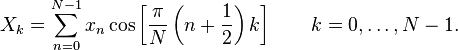
The several occurrences of the data points is expressed in terms of the sum of cosine functions at different periodic frequencies. Cosine functions are chosen over sine functions because of their advantage of efficiency. DCT is quite similar to DFT (Discrete Cosine Transform) but the only difference is that only real numbers are taken into account in DCT whereas DFT takes in complex numbers too.
There are different forms of DCT, which are listed below. Here x,0, …, xN-1 are the spatial coordinates whereas X0 , …, XN-1 are the frequency coordinates. Both are the sequences of real numbers.
DCT-I
DCT-I of N is given by
 where N is a real number greater than or equal to 2,
xn are real and even numbers around n=0 and n=N-1,
k = 0,1,2,…,N-1 and
Xk are real and even numbers around k=0 and k=N-1.
DCT-II
DCT-II is given
by
 where N is a positive real number ( can be less than 2, unlike in
DCT-I)
where N is a positive real number ( can be less than 2, unlike in
DCT-I)
xn are real and even numbers around n=-1/2 and n=N-1/2,
k = 0,1,2,…,N-1 and
Xk are real and even numbers around k=0 and k=N.
DCT-II is the most widely used form of cosine transformation and DCT in general means DCT-II. DCT-II, sometimes also DCT-I is used for compression of correlated pixels in JPEG, MJPEG and MPEG standards. The two dimensional block-based DCT of 8×8 matrix is used for encoding blocks of video. This encoding standard is defined by IEEE 1180 to increase accuracy and reduce mismatch errors.
An example transformation is demonstrated on this figure.
DCT-III
DCT-III is given
by
 where N is a real number,
xn are real and even numbers around n=0 and n=N,
k = 0,1,2,…,N-1 and
Xk are real and even numbers around k=-1/2 and k=N-1/2.
DCT-III can be scaled to get the inverse of DCT-II and therefore is also known as Inverse Direct Cosine Transform (IDCT), since DCT simply refers to DCT-II.
DCT-IV
DCT-IV is given
by
 where N is a real number,
xn are real and even numbers around n=-1/2 and odd numbers
around n=N-1/2,
k = 0,1,2,…,N-1 and
Xk are real and even numbers around n=-1/2 and odd numbers
around n=N-1/2.
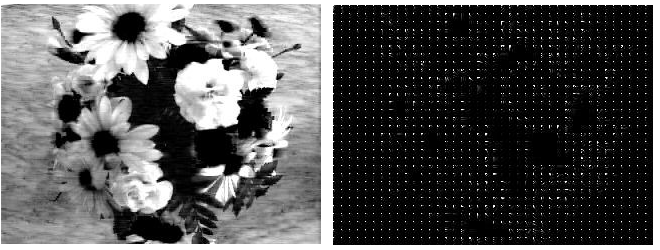 Figure 1.1 : Image and its
DCT coefficients
Figure 1.1 : Image and its
DCT coefficientsQuantization
Quantization is the process of converting a continuous range of infinitely many values into a finite discrete set of all possible values. The quantization process generally approximates the input set into preferably smaller set. The advantage of quantization is that it reduces the number of bits required for storing and transmitting the data. Quantization can be of two types – scalar quantization and vector quantization.
Scalar Quantization
Scalar quantization is a one-dimensional quantization process. It treats
each value from the input set separately.
If the input value be x and output value be y, scalar quantization is
the simple process denoted as:
y=Q(x)
Simple example of scalar quantization is constraining a set of real
numbers into integer values by rounding each real x value to their
closest integer value y. This process is also used in converting analog
wave forms to digital samples.
Vector Quantization
Vector quantization is also known as ‘pattern matching quantization’ or ‘block quantization’. It involves grouping together of input symbols into single units. Grouping enhances optimality of the quantizer but also consumes higher computational resources than scalar quantization. A centroid point is used to indicate a single group or cluster. This kind of quantization is used for lossy data compression of digital data, density estimation and signal processing because it is powerful for detecting density of huge data of high dimensions. For values in vector space of multi-dimensions, quantization encodes them to a bounded set of values from a lower dimensional subspace of discrete nature.
Quantization of Digital Image
Quantization of a digital image is the technique of judging which
sections of the image can be ignored in such a way that the image
doesn’t look significantly different. This is a lossy process. The color
spectrum is also quantized by reducing the number of colors used to
represent it in processes like conversion of
JPEG to GIF since
GIF only supports 256 colors. Quantization is
also done when images are printed because the printers don’t have the
tonal resolution which supports all the colors for all pixels in the
image. Similar is the case with image scanning specially for shadow
areas.
Quantization is a lossy process since it involves approaches like
rounding off and discarding negligible entities. The inverse of
quantization doesn’t produce exactly the same object which was fed for
quantization. Whatever is lost is called quantization noise.
Quantization matrices or quantizers are used for defining the quantization process. Supposing Q[i,j] is the quantizer matrix, every time a matrix of DCT coefficients, say M[i,j], is encountered, it is divided by quantizer matrix Q[i,j] to obtain quantized matrix Mq[i,j]. Here, we are only considering two-dimensional matrices.
The quantization equation can be given as
Mq [i,j] = round( M[i,j] / Q[i,j] )
The inverse quantization equation becomes
M’[i,j]= Mq[i,j] * Q[i,j]
The rounding off is not invertible and therefore the process is lossy.
The loss is measured as quantization error which is given by:
Quantization Error = Mq[i,j] – M’q[i,j]
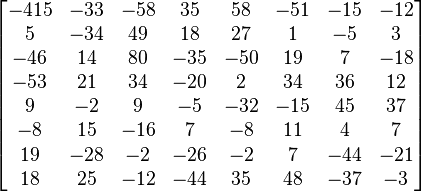
An example:
Matrix of DCT coefficients, M[i,j]=
Quantizer Matrix, Q[i,j] =
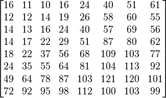
Now dividing each elements from M matrix with corresponding elements (from same row i and same column j) from Q matrix like
Mq[1,1] = round( M[1,1] / Q[1,1] )
= round ( – 415 / 16)
= round ( -25.9375)
= -26
and so on, we get
Quantized Matrix Mq[i,j] =
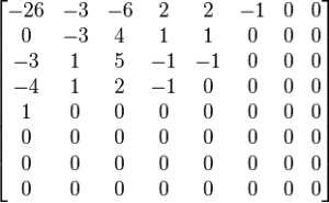
The matrix thus obtained is processed through other techniques like zigzag scanning, entropy encoding etc.
Entropy Coding
Entropy literally refers to the lack of predictability or order. In the context of information theory and engineering, entropy is the measurement of the uncertainty of a variable. Entropy also gives the measure of similarity of dispersion of basic units. Lower is the entropy, higher is the compression. Techniques like statistical forecasting can reduce entropy.
Entropy encoding is the process of ordering the input elements in an optimal way and assigning code for each of them. It is a lossless compression. Entropy encoding can be broken into two steps. The first step is Zigzag scanning and the second one is Variable Length Coding (VLC). The second one has major contribution to entropy encoding.
Zigzag Scan ordering
The most AC values in a quantized matrix are zero. Zigzag scan can be used to gather more number of zeros together. Bringing zeroes together increases the optimality of the encoding process that follows. Zigzag scanning groups the low frequency coefficients before the high frequency coefficients. This processes serializes the matrix into a string.
The 8 x 8 matrix is mapped into a one-dimensional array of 1 x 64 vector. Grouping zeros enables us to encode the bitstream in the pair of ‘skip and value’. Here, ‘skip’ means the number of occurrences of zero and ‘value’ means the occurrence of next non-zero component in the sequence.
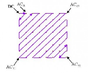
Figure 1.2 Zigzag Scan
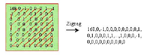
Figure 1.3: Serialization of coefficients with zigzag scanning
Variable Length Coding (VLC)
VLC is the major part of entropy encoding.
VLC is the process of mapping the input
symbols into codes of variable lengths. This enables us to compress the
the symbols without any error. This means the compression is lossless
and decompressing the symbols one by one gives us the same original
input. Compression level close to its entropy can be arbitrarily
achieved if the right coding strategy is chosen. Also, identically
distributed as independent source needs to be selected. Unlike
fixed-length coding techniques, VLC can be
used for compression of small blocks of data too, with less probability
of failure.
Some of the most popular strategies of VLC are
Arithmetic Coding, Huffman Coding and Lempel-Ziv coding.
Huffman Coding
Huffman Coding like other coding techniques for compression is a statistical technique that attempts to reduce the number of bits required to represent a string. The basic idea of this coding technique is to assign a shorted code for the most frequent symbols. Huffman coding algorithm is a greedy process. This technique was introduced by David Huffman (1925-1999) in 1952.The vital part of this coding technique is to generate the codes which are called Huffman codes. Code Book is used to store the Huffman codes. Huffman algorithm is a bottom-up approach.
Huffman code is generated using a binary tree. Such binary tree is
called Huffman tree.
The process of building is tree is outlined below:
Step 1 : Independent parentless node is created for each input symbol,
including the symbol and the probability of its occurrence.
Step 2: The two parentless nodes with the lowest probabilities are
selected.
Step 3: A new parent node is created with the last two selected nodes as
immediate children.
Step 4 : The newly created node is assigned the probability equal to the
sum of its children.
Step 5 : Continue from Step 2 until only only one parentless node
is left.
Thus generated binary tree is unambiguous for decomposing it during decoding process is only possible in exactly one way. Since leaf nodes are used to store symbols, no code happens to be the prefix of another code.
       *
      / \
     (0)(1)
      /  \
    (10)(11)
      / \
    (110)(111)
Context-Adaptive Binary Arithmetic Coding (CABAC) and Context-adaptive Variable-length Coding (CAVLC)
CABAC and CAVLC are coding algorithms used to encode the syntax elements when theprobability of its occurrence in the context is given. These are one of the forms of entropy encoding and are lossless. CABAC has higher compression ratio than CAVLC but decoding a CABAC encoded entity requires more processing than decoding a CAVLC encoded entity. Parallelization and vectorization in CABAC is more difficult than in CAVLC.
Exponential-Golomb Coding
Exponential-Golomb (Exp-Golomb) coding is an alternative for CABAC and CAVLC which provides a more simple yet better structured VLC technique for encoding syntax elements. A non-integer code is used to parameterize the encoding in this process.
Wavelet Transformation
Wavelet transformation is a technique for compression of data used in images and sometimes in audio and video. It is used as a substitute to DCT for transformation of coefficients from spatial domain to frequency domain. Wavelet compression can either be lossy or lossless whereas DCT is always lossless. This is why wavelet may provide more compression ratio than DCT.
Run length Encoding (RLE)
un Length Encoding is a technique of encoding data where consecutively occurring entities are represented only once with a symbol along with the frequency. The original sequence is transformed into a smaller run with data values and their count thus enabling compression. RLE is considered to be one of the oldest data compression approaches. This approach is suitable for all kinds of information, text or binary. RLE may not be suitable for data which do not have items repeating consecutively. RLE can be performed in bit-level, byte-level or even pixel-level in case of images. RLE is a lossless compression.
An example of Run Length Encoding:
Input symbols:
AAHHHHHHHTTTTTTPPPPPWWJKKKKLLLLLLLLLL
Run Length Code : 2A7H6T5P2W1J4K10L
Another example of RLE that only compresses
consecutive zeroes:
Input Symbols : 0000010000000000010001011000000000000
Counting the number of zeroes separated by 1’s,
5 11 3 1 0 12
In 4-bit code representation, the run length encoding is:
0101 1011 0011 0001 0000 1100
Chroma subsampling
In the early years of television broadcasting, same bandwidth were provided for color components and brightness. Soon it was realized that the human perception is more sensitive to intensity than to colors. So, reduction of the resolution of colors or chroma by keeping the brightness or luma intact didn’t alter the picture quality. And then the television broadcasting companies started saving bandwidth by propagating only half the amount of chroma than luma. This methodology they implemented is called chroma subsampling. This is demonstrated in the figure below :
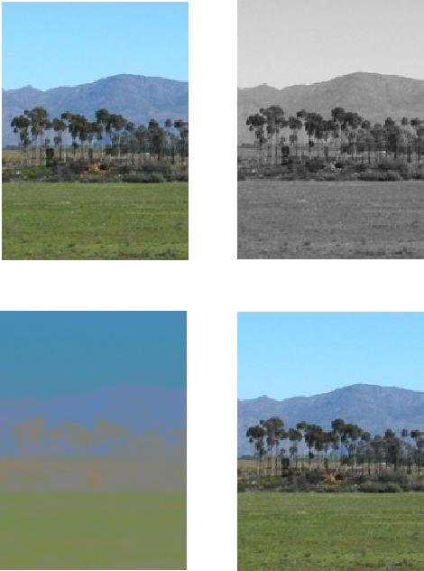
Figure 1.5: Demonstration of color subsampling
Luma, in imaging and video technology refers to the intensity or brightness of the image. It is sometimes called ‘Luminance’ but by convention, the term ‘Luma’ is to be used in video technology and ‘Luminance’ in general color science. Luminance is the weighted sum of the RGB components of image whereas Luma considers the gamma-compressed components- R’G’B’. If Luminance is represented as Y, Luma is represented as Y’, read as Y prime, where the prime (‘) symbol stands for gamma-compression. The weighted sum is calculated by using coefficients that have recommended. Rec. 709 specifies the following expression for computation of luma:
Y’ = 0.212671 * R’ + 0.715160 * G’ + 0.072169 * B’
Chroma, or sometimes called chrominance, is the signal that carries the color information of the image. It is abbreviated as ‘C’ whereas popularly represented as UV, since it is composed of two color-difference components, U and V.
U= B’ – Y’ (Gamma-compressed Blue – Luma)
V = R’ – Y’ (Gamma-compressed Red – Luma)
The Y’UV or YUV color space was used for analog color television systems. For modern digital imaging and video broadcasting the YCbCr family of color spaces are used. Cb stands for blue chrominance and Cr stands for red chrominance. YCbCr color space is not an absolute or basic color space but is an encoding of the RGB color space. Also, like YUV should not be confused with YCbCr , Cb does not correspond to U and Cb does not correspond to V.
Almost all digital video formats today use YCbCr but they vary by the subsampling ratio. The subsampling ratio is generally expressed in the format p:q:r. Popular explanations use j:a:b or H:V:T symbols for the ratio but the bottom-line of all the explanations is the same. The values ‘p’, ‘q’ and ‘r’ are always integers. The first value ‘p’ gives the horizontal width of the sample region or the number of pixels in the row of consideration. It is usually ‘4’ until recently Sony used the 3:1:1 ratio. 4 is used for p for its traditional references and also because being multiple of 2, dividing it for other factors in the ratio becomes easy. So, it’s generally 4:q:r. The second value ‘q’ gives the count of chroma samples in the first row of ‘p’ pixels. So, 4:4:r means there are four chroma samples for a row of four pixels, which implies no subsampling. 4:2:r means there are two chroma samples for a row of four pixels which means the image has been subsampled by the factor of 2. 4:1:r means there is a single chroma sample used for four pixels of the row and thus the image is subsampled by the factor of 4. The third value in the ratio, ‘r’ says only if vertical subsampling has been done. If ‘r’ is equal to ‘q’, vertical subsampling is absent that is same chroma samples haven’t been forced for vertical pixels. If ‘r’ is zero, vertical subsampling has been done for the image.
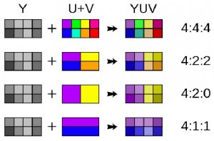
Figure 1.6: Components in different sub-sample ratios
Since pictures and videos are the basic types of multi-media, we now
look into popular
encoding formats of each kind, JPEG and
MPEG.
JPEG
Introduction
JPEG, pronounced ‘Jay-Peg’, stands for ‘Joint Photographers Expert Group’. JPEG is also used to refer to the family of standards this group has created for coding and compression of still images. JPEG standard is the most widespread standard for representation of still images. Images can be represented in other different formats like Bitmap (BMP), Tagged Image File Format (TIFF), Portable Network Graphics (PNG), Graphics Interchange Format (GIF), et cetera. TIFF is mostly used with Optical Character Recognition, and GIF is popular with animation (not still images). Lossless PNG files are preferred for editing images whereas JPEG is usually preferred for distribution because of its great compression abilities which makes it more portable and yet with considerable quality despite being lossy.
JPEG is the most widely used and a very flexible digital photograph compression standard. It is the best example of continuous tone image compression technique. Continuous tone is the term used for images in which each color at any point is independent color or single tone from its surrounding points and the quality of the image depends on how many points are there in given size of image. JPEG is lossy image compression method where the size of image and its quality is inversely proportional. JPEG compression technique can withstand compression ratio of 10:1 without compromising with quality noticeably. There is an alternative standard for image compression which is not used widely and not compatible across variety of devices.
JPEG, technically, is a compression method whereas the file format is defined to be JFIF (JPEG File Interchange Format). In general usage, JFIF files are called ‘JPEG images’ and are represented with file extensions – .jpeg, .jpg, .jfif, .jfi. The MIME type for JFIF file format as specified in RFC 2046 in 1996 is ‘image/jpeg’. A JPEG file has the bytes ‘FFD8′ in its beginning and ‘FF D9′ at its end. ‘4A 46 49 46′, which is the ASCII code for the string ‘JFIF’ is used as a null terminated string in JPEG/JFIF files.
JPEG Standardization Body
Joint Photographers Expert Group is a joint committee of the standardization bodies ISO/IEC JTC 1 and ITU-T (International Telecommunications Union). ISO/IEC JTC 1 in turn is the joint committee of ISO (International Organization for Standardization) and IEC (International Electrotechnical Commission). In fact, JPEG is just a nickname to this joint group. The official homepage of the group is http://www.jpeg.org. The committee meets at least three times a year and has been publishing parts of the JPEG, JPEG-LS, JPEG 2000, JPSearch and JPEG XR standards.
History of JPEG
The first JPEG standard – JPEG Part 1 was published in 1992, which explained the requirements and guidelines for digital compression of images. JPEG Part 2 released on 1994 explained compliance testing and JPEG Part 3 released on 1996 explained the extensions. JPEG Part 4 released on 1998 added profiles, index tags, color spaces, markers and other designations to JPEG. JPEG Part 5 is under development and in a recent press release, the joint group has revealed that JFIF will be standardized and designated as JPEG Part 5.
JPEG-LS is the standard for lossless or near-losless compression. Part 1 and Part 2 of this standard were released in 1998 and 2002, which specified the baseline and the extensions of the standard, respectively. The group has also published MRC (Mixed Raster Content) in 1999 which is used for image segmentation. Six parts of JPSearch standard has been released starting from 2007, of which Part 2, 5 and 6 still being under development. JPEG XR standard has five parts published, Part 1 surprisingly being the latest one to be revised. Also, the group is developing AIC (Advanced Image Coding) with major involvement from ISO/IEC.
‘JPEG 2000′, not to be confused with the JPEG standard, is another image compression standard the group has been publishing since 2000 and its Part 14 is currently under development.
Compression in JPEG Standard
Psychovisual Compression
The human perception is not highly sensitive to detailed spatial information. This means our vision has limited response to details around edges of objects and shot-changes. This nature of human perception can be exploited to reduce the amount of information in an image or video frame and thus allows some considerable amount of compression without real significant notice.
JPEG makes use of Chroma Subsampling as a psychovisual compression technique. This technique exploits the fact that human eye is far less sensitive to the variation in hue than that in brightness. JPEG utilizes the 4:2:0 and 4:1:1 subsample ratio, 4:2:0 being the usual one.
Spatial Redundancy Removal
Block preparation is the first step of the compression. Blocks of 8 x 8
pixels are segmented. A block then can be represented in a 8 x 8 matrix.
The spatial variation of pixels in each matrix is converted into
frequency variations using two dimensional Discrete Cosine Transform.
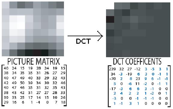 Figure 2.1 : Transformation of 8 x 8 picture matrix to
DCT coefficients
Figure 2.1 : Transformation of 8 x 8 picture matrix to
DCT coefficientsWavelet Transformation may also be employed as a substitute to DCT, although it is more widely used in the JPEG 2000 standard. DCT is always lossless whereas wavelet may be lossy. Quantization is performed over the retrieved transformation coefficients to convert higher frequency coefficients into zero. Some insignificant amount of information is lost during this process. The quantized matrix then entropy coded. The DC component of the matrix is encoded using DPCM (Differential Pulse-Code Modulation) which is a derivation of the PCM (Pulse Code Modulation) technique. DPCM uses the differential value among the sample nodes for coding. Whereas for the AC coefficients, zigzag scanning is done to align zeroes on one corner. Since zeroes are accumulated at the end, End of Block (EOB) marker can be used to replace the final run of zeroes, which further reduces the bit-size. Run length Encoding (RLE) is applied to reduce the redundancy. Then, Huffman Coding or Arithmetic coding is to be done to get smaller array of data. Although JPEG standard recommends any of these two Variable-Length Coding (VLC) to be used, Huffman Coding is preferred for its better compression. VLC is the last step during encoding and first step during decoding of JPEG images.
Decoding of JPEG
Decoding of JPEG file is the inverse process of its encoding. The decoding process starts with entropy decoding. Variable-Length decoding is done. Huffman Code Book is used for identifying the symbols for which the codes are used. Inverse quantization and then Inverse DCT (which is DCT-III) further decodes the image file. This gives us a very very close match of the raw image that was fed to the encoder. The decoding process requires information about how the encoding or the compression has been done. This information is available within the JPEG file as CH (Compression History).
JPEG Compression Modes
There are four modes of JPEG compression:
Lossless JPEG
Lossless JPEG compression mode uses only predictive technique. No information is discarded if it isn’t redundant. Entropy coding is employed for this no quantization is done. Eight kinds of prediction schemes are used.
Baseline or Sequential JPEG
This is the most common mode of JPEG compression. It employs all the lossy and lossless compression algorithms for psychovisual compression as well as spatial prediction. It involves chroma subsampling, DCT, quantization and entropy encoding.
Progressive JPEG
Progressive JPEG is a lossy mode and is very much similar to the baseline JPEG except that multiple scans are done for coding. It is of two kinds – spectra selection and successive approximation. Some applications use image/pjpeg MIME type for images compressed with this mode. It is suitable for download in slower internet connection where portions of the images can be gradually downloaded.
Hierarchial JPEG
This is a lossless mode based on DCT. Multiple frames of differential and non-differential kinds are used. This mode provides multiple resolutions and the images compressed with this mode take more space.
Applications of JPEG format
Digital photography is primarily used for sharing information and storage. JPEG images are widely used for sharing images in internet. Besides just photographs, thumbnails for pages, videos, and other different contents are encoded as JPEG. JPEG is suitable for all kinds of devices – powerful computers as well as mobile devices of low end. It is also appropriate for sharing in all kinds of connections. The capability of level wise compression with minimum loss in the quality of JPEG compression standard makes it very popular and applicable. JPEG is preferred as widely used image compression standard because it is capable of storing 24 bit per pixel color data instead of 8 bit per pixel color data which were used before.
JPEG is the format used for saving images in digital cameras, storing them, as images in web-pages and everywhere else. The image in ID3 tag of MP3 files for album covers and artist pictures are also encoded as JPEG images.
Another use of digital photographs is for scientific research and medicine. Scientists and doctors can share their findings, results and problems between each other for better consequences. These can be stored for future also so that future generations of scientists and doctors can study them. In such cases the size of the image wont matter as such but the quality has to be very good. They can zoom in and magnify the minute details which would have been impossible to detect by the normal human eye. Such super high quality of images is supported by JPEG.
Capturing the personal moments in the form of still photographs is very important as well. In this age of web 2.0 where idea of sharing pictures of what you are doing now to your important friends and families to get connected with each other and remember the moments of personal, cultural and social events is very important as well. JPEG is the best choice for this purpose.
Digital imagery are also used for surveillance and better representation of raw data in the form of information. Maps make our day to day life easier. These are only the few examples of implementation of Digital Photography and JPEG compression standard to be specific.
JPEG’s Limitations
JPEG has some downsides too. It is a lossy compression standard. It may not be appropriate in cases where the minute details of the image and high quality precision matters more than the storage size and transmission bandwidth. JPEG can easily handle compression ration of 10:1 without drastically degrading the quality but this is also disadvantage of the JPEG as it takes longer time to decode or decompress. There always has to be a compromise between time and space. There is already a new and improved standards of JPEG family called JPEG2000 but the transition to this new format is becoming very difficult as very low number of device so only very few improvements have been made in past two decades and there is no sign of that transition happening very soon.
JPEG is superior when we need rich colored and realistic photograph since it supports 24 bit per pixels but when the quantity of colors of the photograph is lower, it creates overhead and cannot compress as good as other image compression standard like GIFs. Another limitation of JPEG file format is that it cannot handle transparency and very sharp edges.
Future Technologies of JPEG
Joint Photographic Expert Group (JPEG) in 1992 introduced a very popular image compression algorithm and standard called JPEG. It is true that JPEG has been one of the most reliable and easy to use photo standard and thus it is the most popular also but very little improvements have been made by the group since last two decades. Technology needs constant revisions and improvements but JPEG committee instead of improving the existing standard introduced a new photo compression and coding algorithm that is meant to replace JPEG. This standard is called JPEG2000, which was introduced initially in the year 2000. JPEG2000 itself is based on wavelet method and there are two standard file format ‘.jp2′ and ‘.jpx’ . Although its been a decade since JPEG2000 was first introduced people have not accepted the file format. It is also thought that JPEG2000 is only a modest improvement to existing JPEG compression standard so until there is something very revolutionary there is no need to totally shift to new technology.
Now JPEG2000 is the improved standard of photo compression from Joint Photographic Expert Group committee itself but there are lots of other versions of JPEG that have been standardized and are in the development process. Examples of such is JPEG XR where XR stands for eXtended Range and JPEG Mini. JPEG XR is also compression standard for still photographs and digital graphics which is based on technology which is developed by Microsoft under HD Photo standard. Although JPEG XR is a standard that improved the deficits of JPEG but then JPEG XR is not a open standard and patented by Microsoft and so there are very few vendors who support this standard like Microsoft itself and Adobe. There are bunch of other so called improvements to JPEG that are either waiting to be standardized internationally or adopted by peoples. The JPEG mini which is also developed by independent Israeli group is compatible with existing JPEG and compresses the images 5-10 times more without losing the original quality. It can be said that this is in very infant stage and still need some improvements.
MPEG
Introduction
MPEG, pronounced ‘M-Peg’, stands for ‘Moving Picture Experts Group’. Like JPEG, MPEG can be used to refer to the group itself or the standards the group has created for coding audio-visual data. There are various digital video encoding formats or codecs, among which some popular ones are 3GPP (popular on mobile phones), AVI (Microsoft’s Audio Video container codec derived from RIFF), FLV (Flash Video, popular on web pages, utilizes Adobe Flash Technology), MOV (Apple’s QuickTime multimedia format), etc. While these formats have their own special capabilities and abundance in particular platforms, codecs from the MPEG family are the most widespread and accepted ones. The official homepage of MPEG is http://mpeg.chiariglione.org/ whereas resources and references are available on http://www.mpeg.org.
MPEG files are generally represented with the extension ‘.mpg’. Its MIME type is ‘video/mpeg’.
History of MPEG
With an objective to provide better quality videos with small file sizes, ISO, IEC , SC2 and few other organizations initiated the movement in January 1988. The following table gives an overview of the early phases and the MPEG-1 and MPEG-2 development.
| Date | Place (if meeting) | Description |
|---|---|---|
| May 1988 | Ottawa, Canada |
First official meeting. Relate motion video to digital storage devices. Real-time decoding at bitrate of 1.5Mbit/s. |
| 18-22 July 1988 | Politecnico di Torino, Italy | IVC (Internet Video Coding) and CDVS was proposed |
| September 1988 | London, UK | Goals and objectives were hammered. |
| December 1988 | Hannover, Germany |
Audio coding activity initiated. Video testing sequences were selected by video group. |
| February 1989 | Livingston, New Jersey, USA | Techniques for matrix testing were specified |
| June 1, 1989 | - | Deadline for audio standard development participation. |
| May 1989 | Rennes, France | Dedicated meeting for description of proposal packages. |
| July 1989 | Stockholm, Sweden |
Finalization of video package. Initiation of activities on MPEG system. |
| October 1989 | Kurihama and OSaka, Japan | Proposals for decompressed digital image sequences were made available. |
| January 1990 | Eindhoven, Netherlands | Semi-independent testings were made possible by core experiments. |
| March 1990 | Tampa, Florida, USA |
Results from core experiments were analyzed. JPEG vs. H.261 comparison was run for picture coding. Syntax in pseudocode was defined. SM1 (First Simulation Model) for video was bring forth. |
| April 1990 | Washington, USA | Working Group – WG8 was restructured. |
| May 1990 | Torino, Italy | MPEG-2 with high definition coding was proposed. |
| September 1990 | Santa Clara, California, USA |
Macroblock level was selected for motion compensation. WD (Working Draft) was created. |
| December 1990 | Berlin, Germany |
MPEG-1 standard (WD
11172) was edited. Requirements for MPEG-2 were specified. |
| March 1991 | San Jose, California, USA | Meetings canceled due to Gulf War crisis. |
| May 1991 | Paris france | WD 11172 was edited and cleaned up. |
| August 1991 | Santa Clara, California, USA | MPEG-1 WD was prepared to promote to CD (Committee Draft). |
| November 1991 | Kurihama, Japan | MPEG-1 WD was accepted as CD. |
| January 1992 | Haifa, Israel | WG11 created DIS (Draft International Standard) 11172. |
| July 1992 | Angra dos Reis, Brazil | TM1 (Test Model 1) for MPEG-2 was made available. |
| September 1992 | Tarrytown, New York, USA | Discussions with cable companies for likely application of MPEG-2 for cable television. |
| November 1992 | London, UK |
First WD for
MPEG-2 was created. It was realized that MPEG-2 could fulfill what MPEG-3 was expected to. |
| January 1993 | Rome, Italy | Technical details for MPEG-2 were worked out. |
| April 1993 | Sydney, Australia |
Main profile of MPEG-2 was frozen. Macroblock stuffing was discarded. |
| July 1993 | New York, USA | Started to clean the scalabilty aspects of WD. |
| September 1993 | Brussels, Belgium | Cleaning up of scalabilty continued. |
| November 1993 | Seoul, Korea | MPEG-2 CD 13818 was published. |
| March 1994 | Paris, France | DIS 13818 was prepared. |
| July 1994 | Norway | MPEG-2 Part 6 (DSM CC) was published. |
| November 1994 | Singapore | MPEG-1 and MPEG-2 achieved final approval. |
Standards of the MPEG Family
MPEG-1
MPEG-1 was designed for encoding multimedia with videos of VHS (Video Home System) quality and audio of bit rate up to 1.5 Mbit/s. MPEG-1 standard, specified as ISO/IEC 11172, has 5 parts, viz. Systems, Video, Audio, Compliance testing and Software simulation. This standard is highly influenced by the standards JPEG and H.261 developed by ITU-T. Resolutions up to 4095×4095 and bitrate up to 100 Mbit/s is supported by MPEG-1. 4:2:0 color space is only supported. Audio, part 3 of MPEG-1, defined as ISO/IEC-11172-3, is the first standard audio compression technology. It only supports two channels of audio. It is divided into three layers – Layer I, II and III.
MPEG-1 Layer III is commonly known as MP3.
MPEG-1 can compress video in 26:1 and audio in
6:1 ratio without significant notice in
degradation of quality.
MPEG-1 had following weaknesses which gave
birth to the next standard:
• MPEG-1 had no standard support for
interlaced video.
• Audio compression is possible with only two channels.
• Only ‘4:2:0′ color space is supported.
• Not compatible with videos of high resolution.
MPEG-2
MPEG-2 is is the most popular standard for video compression with huge range of applications. It was extended from MPEG-1 with lots of improvements and feature additions. It goes up to Part 11, Part 8 (10-bit video) being dropped. MPEG-2 Part 3 (ISO/IEC 13818-3) which describes Audio is backward compatible with MPEG-1 Audio whereas Part 7 describing AAC (Advanced Audio Coding) is not. MPEG-2 adds Variable quantization and Variable Bit Rate (VBR) to MPEG-1 among other features. Since, MPEG-2 has more complex algorithm for encoding, MPEG-1 is slightly better for compression of videos with low bit rates. MPEG-2 can produce compression down to the bit rate of around 3-15 Mbit/s. Any lower bit rate than this may introduce noticeable impairments in the video.
MPEG-3
MPEG-3 was expected to be the standard for high definition television but it was realized that MPEG-2 was capable of fulfilling the need with extensions and therefore MPEG-3 doesn’t exist as a coding standard.
MPEG-4
In early 1995, development of the next standard was initiated so that low bit rates could also be supported. This standard was called MPEG-4 and it reached CD (Committee Draft) status only in March 1998 and the final approval was obtained in the end of the same year. Since then, twenty seven parts of MPEG-4 standard has been published while Part 28 is under development. However, MPEG-4 is not limited to videos with low bit rates, it is becoming the generic standard for video coding.
MPEG-4 employs object-based compression technique which endorses more efficient and scalable compression with wide range of bit rates. The object-based interaction also enables developers to control each objects of a scene independently and also enable the interactivity among the objects. MPEG-4 Audio or as it was specified as ISO/IEC 14496-3 determines the audio coding and composition standards with support for very low to high bitrates. Audio components are also objects which have natural and synthetic quality.
MJPEG is not to be confused with MPEG. MJPEG nothing but a sequence of image frames that uses JPEG compression for each frame.
Video Fundamentals
Video is the technology in which moving visual images are recorded, reproduced and/or broadcasted. An analog video is a video with uninterrupted time varied signal. A digital video is composed of sequence of still digital images. Such still images are called video frames.
Frame rate is the frequency in which consecutive still images appear in a video. It is measured in fps ( frames per second).
An interlaced video is a video with interwoven frames. Frames are interwoven with fields. Each frame has two fields (or half-frames) – odd fields and even fields.
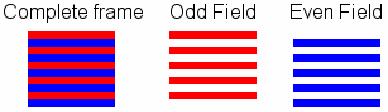
Figure 3.2 : Frame and its fields
Video Object (VO)
A video object is any arbitrarily shaped object, a rectangular frame or
the background scene of a video. A video object can be accessed and
manipulated by the user. A user can browse or seek the video objects
while accessing the video and cut or paste the video objects while
manipulating it.
Video Object Plane (VOP)
Video Object Plane is the instance of Video Object at a given time. It
may also be defined as time sample of video object. A
VOP of rectangular shape forms a conventional
video frame. A video is made up of such encoded VOPs.
Group of Video Object Planes (GOV)
A collection of video object planes is called Group of Video Object
Planes or GOV in short. GOVs are not mandatory
in videos. Random Access points in video bitstream is facilitated by the
points provided by GOVs. One of the reasons video objects are grouped
into GOV is that redundancy can not only be
removed from objects but from the whole group.
Video Object Layer (VOL)
A Video Object Layer is the representation of video objects in single or
multiple strata. A VOL with single stratum is
in non-scalable form whereas a VOL with
multiple strata is a scalable form.
Frames
MPEG identifies frames into three kinds:
1. I-frames
2. P-frames
3. B-frames
Each one of these frames has different properties and purposes, as explained below.
I-frames
I-frame is short for intraframe or intra-coded frame. It is also called keyframe as it is the most important kind of frame. It is independent since this frame doesn’t need other frames for being decoded. It contains more amount of bits or information compared to other kind of frames and therefore is the least compressible, thus taking more storage and bandwidth. The more I-frames a video has, better is its quality.
P-frames
P-frame is the short name for predictive frame or predicted frame. P-frames depend on preceding I-frame or P-frame for information like content and color changes, thus the name predictive. It is more compressible than I-frames.
B-frames
B-frames means bidirectionally-predictive-coded frames frames or simply bi-directional frames. Bi-directional frames do not include information contained in preceding or following I-frames or P-frames and thus depend upon previous and next frame during decoding and decompression and thus the name bidirectional. It provides highest level of compression compared to the other two kinds of frames. B-frames are never reference frames.
Since P-frames and B-frames only store the changed information relative
to the other
frames, they are also known as delta frames.
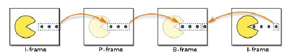 Figure 3.3: An example frame sequence in videos
A Group of Pictures is a collection of frames. A GOP (contains at least one I-frame. In an averagely compressed NTSC video, usually every 15 th or so frames are I-frames although the MPEG standard isn’t strict about this. A GOP may look like IBBPBBPBBPBB, where I stands for I-frames, B for B-frames and P for P-frames. The arrangement of frames determines the GOP structure which is ultimately one of the factors for determining the compression ratio.
Open GOPs and Closed GOPs
Open GOPs are the GOPs which contain frames that can refer to the frames
from preceding or following GOPs. I contrast, delta frames in closed
GOPs can only refer to its own I-frames. Among open and closed GOPs of
same number of frames, open provides a little more compression since
open GOPs contain one less P-frame and one more B-frame than closed
GOPs. However open GOPs aren’t applicable to all
MPEG streams like mixed-angle or
multi-angle DVDs.
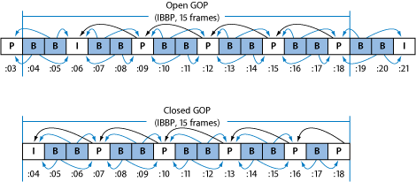 Figure 3.4: Comparison of Open and Closed GOPs
Macroblock
A macroblock (MB) is a segment or component of frame. 16×16 blocks of pixels are usually taken as a macroblock where as 8 by 8 pixels for advanced prediction mode. A still image or video frame contains several non-overlapping macroblocks. Macroblocks are the basic units of consideration in motion estimation and compensation. They are also used used for motion vectors for predictive coding of frames, that is for finding the difference between two frames. A series of macroblocks forms a slice.
Compression
Psychovisual Compression
Psychovisual compression on MPEG is done similarly as in JPEG with Chroma subsampling.
MPEG usually utilizes the 4:2:0 sub-sample configuration in most of its implementations like DVDs, etc. Also, MJPEG’s common implementation includes 4:2:0 configuration. MPEG also utilizes 4:1:1 subsample pattern. NTSC videos in DVCPRO, DV and DVCAM use this pattern. The 4:4:4 subsampling can found in MPEG-4 Part 2 and MPEG-4 since it is considered to be a high quality sampling scheme.
Spatial Compression
I-frames being independent frame are simply just still pictures. Spatial redundancy removal is an intra-picture compression technique. Spatial meaning relating to space, this technique is concerned with removing redundancy over the space of two dimensional plane and not the time dimension. It takes advantage of the fact that a pixel value can be predicted from its neighboring pixels to some extent. Also, human eye is not capable of detecting small changes in the image. This removal technique is also known as backward prediction. This prediction is done within an I-frame and does not depend upon information in preceding or following frames. This kind of prediction is also known as backward prediction.
Compression/Encoding of I-frames
An I-frame is chambered into different macroblocks , say of 8 by 8 blocks of pixels. The macroblocks are then transformed using Discrete Cosine Transform which results in a 8×8 matrix of coefficients. This transformation is not lossy which means the inverse of cosine transformation gives us the original block. DCT-II, sometimes also DCT-I is used for compression of correlated pixels into frequency variations. The two dimensional block-based DCT of 8×8 matrix is used for encoding blocks of video. This encoding standard is defined by IEEE 1180 to increase accuracy and reduce mismatch errors.
Wavelet compression may also be employed in
MPEG-4 technology as a substitute to
DCT. Quantization of the frequency variations
is performed during the process of which many coefficients, generally
the coefficients with higher frequency are changed to zero. This
quantization is a lossy process, which means the inverse transformation
of the quantized matrix gives a similar matrix but not the original one,
however, this doesn’t significantly alter the image quality. Non-linear
quantization of Direct Cosine coefficients is also possible with
MPEG-4. MPEG-4
employs Twin Vector Quantization (VQF) which
considers time domain as one of the dimensions. The matrix of quantized
matrix is then itself compressed to obtain zeros on one corner of the
matrix. Zigzagging is performed beginning from the corner opposite to
where the zeros have been aligned. Zigzagging combines the coefficients
into a string. The redundant consecutive zeros from the string are
substituted with run-length codes which is the popular Run length
Encoding (RLE) algorithm. Huffman Coding is
then applied as a VLC to obtain smaller array
of
numbers.
H.264/MPEG-AVC employs Context-Adaptive Binary Arithmetic Coding (CABAC) and Context-adaptive Variable-length Coding (CAVLC) for variable-length coding. CABAC is used whenever higher compression is required and CAVLC is used in slower playback devices to increase the performance since it is a lower efficiency scheme. All H.264 profiles support CAVLC whereas only Baseline and Extended profiles do not support CABAC. So CAVLC support is seen everywhere in in all kinds of decoders like Blu-ray and HD DVD players. CAVLC is also supposed to be a superior technique than DivX, XviD and other MPEG-4 ASP codecs. Although CAVLC may be used for coding transform coefficients, Exponential-Golomb Coding is used to code other syntax elements in the video stream.
Decoding/Decompression of I-frames
The I-frames in MPEG video are required to be decoded in order to be played by the media player or the video broadcast receiver (e.g. television). The decoding process is more or less the inverse of the encoding process. The decoding process starts from the Huffman Decoding. Then Run Length Decoding is performed and the result is fed for Inverse Quantization. Quantization process being a lossy one, the matrix after inverse quantization during encoding is not exactly the same as the matrix before quantization during the encoding process. The inversely quantized matrix is then passed through Inverse Discrete Cosine Transform (IDCT) to obtain the macroblocks. The macroblocks are structured to obtain the I-frame which is very much similar to the I-frame where the compression started.
Temporal Prediction
Temporal prediction takes advantage of the fact that neighbor frames in a video have similar information. Temporal meaning relating to time, temporal redundancy removal is concerned with representing repeating information in consecutive or close frames only once by employing different algorithms. Temporal prediction involves coding of P-frames and B-frames.
Temporal compression provides more compression than spatial compression as seen on I-frames, because very small information is required to specify the minor changes between the frames. Objects may differ with shift in position, rotation or intensity and the new object can be created just by knowing how different is it from the original object. Storing the original and changed object takes a lot more space than storing the original object and and just the difference.
Encoding of P-frames and B-frames
Encoding of P-frames and encoding of B-frames are similar except that
P-frames refer to the information in the previous I-frame or P-frame and
B-frames refer to both the previous and next frames. As the first step,
the previous frame is reconstructed for P-frame encoding and both
previous and next frames are reconstructed for encoding of B-frames to
obtain reference frame. The frame to be compressed is
then segmented into macroblocks, say of block size 16
by 16 pixels. The reference frame is
searched for best match of the macroblocks for each
macroblocks of the frame being compressed. Exhaustive search, 2-D
Logarithmic search, or Three-Step Search (TSS)
may be used to optimize the search. For most of the macroblocks, an
exact match is found on the reference frame because two subsequent
frames have very less change in their blocks. Since some components move
in the frames, offset is calculated. A component may be
moving 15 pixels to the right and 9 pixels up. Such
offset or shift is represented as ‘motion vector’,
which is a two-dimensional vector. The offset and the motion vector is
frequently zero because most blocks in subsequent frames are consistent.
Offset value is not always enough to describe the change in frames
because sometimes not just the placement of macroblock changes but their
appearance too. This change can be measured by taking into account each
pixels of the two macroblocks and
finding the difference between corresponding pixels.
The difference is computed as coefficient values which is then obtained
as string called residual. This residual value
undergoes compression. The residual value which is in
spatial domain is transformed using DCT of two
dimensions. The transformation coefficients are then quantized to reduce
their bit size, most of them quantized to zero. The quantized
coefficients are passed through entropy coding for further compression.
The final information is then combined with the motion vector along with
other information like frame types, etc. to obtain the final difference
known as prediction error between the frames.
The above explained method is the most common method of motion estimation indifferent video coding standards, also seen on MPEG. This technique has been given several names such as Block-Matching Algorithm (BMA) or Block Matching Compensation (BMC). This block-based method utilizes algorithms like Mean of Squared Error (MSE), Matching Pel Count (MPC), Mean of Absolute Difference (MAD), Sum of Absolute Difference (SAD), etc. SAD is used in MPEG technology to get the variation of macroblock matches using polygons of modified blocks.
Instead of basing the blocks on integer values, half-pels can also be taken as the basic unit which may increase the compression ratio but this eats a lot more computational resources. Several other methods exist for motion estimation and compensation like Pel-Recursive Algorithm (PRA), phase correlations, Bayesian estimations, etc. But block-based compensation is believed to be the most efficient one.
Older MPEG standards use fixed block size for
the motion estimation and compensation process. Newer standards like
MPEG-4 Part 2,
MPEG-4 AVC use
dynamically selected size of the blocks. This method is known as
variable block-size motion compensation (VBSMC). This enables the encoder to use larger or smaller block size
whichever is more efficient. Larger block size can decrease the bits
required to represent the motion vector whereas smaller block size may
allow for more precise prediction error.
MPEG-4 even allows wavelet transforms instead
of DCT during the conversion of spatial
variations to
functional variations.
Decoding of Delta Frames
Encoding of delta frames, i.e. P-frames and B-frames involves computation of delta factors which are the displacements of macroblocks and the residual values. During the process of decoding these factors are applied on the reference frame to obtain the candidate frame which can then be displayed. Since the residual value goes compression during encoding it has to be decoded using entropy decoding, inverse quantization and IDCT. This decompressed coefficient of residual and the motion vector gives the prediction error or difference between reference and candidate frame. So, adding this difference to the reference frame gives us the required candidate frame which is not exactly the same frame before encoding due to lossy algorithms used but is of considerably good quality.
MPEG videos are not suitable for editing because of the presence of the reference frames since P-frames and B-frames depend upon I-frames and other P-frames for being decoded. Cutting a frame could break other frames which depend upon it. Formats specially created for editing videos keep all frames as independent I-frames. The interdependence of frames is also the reason why all MPEG decoders are forced to have encoders built in within themselves.
Compression of Audio
Audio in MPEG is compressed with techniques like sub-band filtering, psychoacoustic model and quantization of digital audio. Audio signals are divided into frequency sub-bands using convolution filters. There are 32 critical sub-bands available. Psychoacoustics utilizes the aspects and processes like limits of perception, masking effects and sound localization.
Quantization of Digital Audio
Quantization of digital audio means converting of sound waves to a distribution of individual samples each having unique magnitude of amplitude. Bit depth is what is used to define the range of levels of amplitude. An 8-bit quantization means there are total of 256 possible values for the amplitude levels whereas 16-bit quantization means there can be total of 65,536 possible values of amplitude. Autocorrecting music tracks is also done with quantization in which the beats are distributed evenly to remove errors on timing by analyzing and stretching in time.
MDCT (Modified Discrete Cosine Transform) is a variant of DCT-IV in which the various transforms are overlapped. MDCT is used in audio compression in the MPEG-1 Audio Layer 3 and MPEG-2 Audio Layer 3, i.e. MP3 as well as in AAC and Vorbis encoding.
VBR and CBR
With VBR (Variable Bit Rate), higher bit rate may be assigned to the segments with higher complexity of audio or video file and lower for less complex segments. The bitrate for the whole file is represented as the average bitrate. In contrast, in CBR (Constant Bit Rate), all segments are given the same bit-rate. VBR provides more flexibility, accuracy and quality whereas CBR provides more compatibility with devices, software and connections.
Implementations of MPEG
Codecs
Most televisions, multimedia players have support for decoding MPEG. Several codecs are available for different operating systems. A codec (compressor-decompressor) is a software or hardware that can encode/compress and/or decode/decompress digital stream of data. A software codec may not be a stand-alone program but just a library or module. Xvid is an example of codec which is the open-source codec that implements the MPEG-4 standard. FFmpeg is one of the most popular projects for producing free audio/video codec libraries for MPEG. Interestingly, FFmpeg uses this zigzag pattern used for entropy encoding of MPEG videos in their logo.
 Figure 3.5: FFmpeg Logo showing zigzag pattern
MP3
MP3 is a popular name for MPEG-1 and MPEG-2 Audio Layer III. It is the most widely used audio encoding format. MP3 standard was finalized in 1992 and released in 1993. MP3 is a lossy format. It supports both CBR (Constant Bit Rate) and VBR (Variable Bit Rate) encoding. MP3 files usually have ‘.mp3′ file extension and their standard MIME type is ‘audio/mpeg’. MP3 has support for ID3 and other kinds of tags for storing metadata and DRM information of the audio file. The MP3 encoding format is patented. MP3 is the most popular audio file format and is used for music tracks, online streaming, audio recording, etc.
MP4
MP4 is a common name for MPEG-4 Part 14. MP4 is a container for digital video and audio streams. MP4 files can also contain subtitles, images and hint tracks. The hint track is what makes MP4 easily possible to be streamed over the internet. MP4 encoding is specified in the standard ISO/IEC 14496-14. It is heavily influenced from the QuickTime File Format. MP4 files are represented with the file extension ‘.mp4′.
Applications of JPEG
MPEG, being the most popular video coding standard, has very wide range of applications.
Television and Broadcasting
All terrestrial, cable or broadcasting television technologies like DBS (Direct Broadcast Satellite), DVB (Digital Video Broadcasting), ISDB-T, HDTV (High Definition Television), CATV (Cable Televisions) depend on MPEG. Most terrestrial television systems use MPEG-2 although some use MPEG-1 for certain purposes. ATSC (Advanced Television Systems Committee) have also standardized MPEG-2 as the official encoding format. Smart Television systems like Apple TV also support MPEG-4 video up to 2.5 Mbps.
Internet, Mobile, Multimedia and Gaming
MPEG is also very popular with online streaming. Since bandwidth is an important factor in internet, MPEG format is usually chosen for its better compression. It is also gaining more popularity in mobile multimedia because of its smaller size. Motion pictures in most video games are also rendered using MPEG.
Recording and Communication
Varieties of digital camcorders and video recorders use MPEG as the default format for recording videos. Products like XDCAM implement in the standard in their own different ways. Different communication activities like video conferencing and video calling also utilize MPEG.
Storage and Distribution
MPEG-1 is used for VCDs (Video CDs). The very popular DVD videos are possible only because of MPEG-2. The latest Blu-ray technology also utilizes MPEG-2 Part 2 and H.264/MPEG-4 AVC.
Limitations of MPEG
Newer standards of the MPEG family keep being
published to overcome the limitations of the older one. The latest
popular standard has many limitations. The current downsides of the
format have been listed below:
• MPEG being a lossy compression doesn’t
preserve all minute data.
• The compression flow involves many encoding and transformation
algorithms which could be difficult to perceive and implement.
• AAC and OGG Vorbis
provide better audio encoding than MPEG audio
layers.
• MPEG is not the best file format for online
streaming and therefore is slowly
being replaced by other file formats like
FLV (Flash Video).
• Overlapped Block Motion Compensation (OBMC)
is not allowed in profiles in all parts of
MPEG-4 standards.
• MPEG-4 has a short header format.
• Initial parts of MPEG-4 couldn’t provide
significant improvement in bit-rate that caused users to be attracted to
other encoding formats.
• Since MPEG is a patented format, non-free
MPEG encoders and decoders may be subject to
royalty fee.
• End-users may have to bear the royalty when using free software like
VLC for encoding and decoding purposes.
Future of MPEG
Huge improvements in video encoding have been made since the introduction of MPEG-1. Every new specification released gives better compression of data and allows more features for video technology. The latest widespread standard MPEG-4 provides lot more flexibility with support for internal subtitles and hint tracks. Online streaming and other certain needs of the modern days may be fulfilled by it is not the most optimal format. It requires lot more improvement to win back the video streaming in internet from other encoding formats like FLV. With booming of Internet and Smart TV systems like Google TV and Apple TV which promise to provide a lot more flexibility for the users, a better standard is required as the currently standardized specifications of the MPEG family may not be enough to support this flexibility. Also, with portable devices gaining more popularity, the standard has to be portable with easy support for wide array of devices. MP4 may be replacing mobile video coding technologies like 3GP but it has a lot more space for improvement. Use of MPEG is not appropriate for all gaming and interactive contents. More profiles have to be added to the standard. Also, there is a room for better compression in audio.
MPEG-4 Part 28 which is under development has lots of improvements to bring. MPEG DASH led by employees of Microsoft is also believed to overcome many limitation of MPEG-4, as a common adaptive-optimized encoding format. Despite being one of the most popular video encoding standard, MPEG falls short in may applications and its future is uncertain unless huge improvement and flexibility have been added to it.
REFERENCES
William B. Pennebaker, Joan L. Mitchell, 1992. JPEG: Still Image Data Compression Standard (Digital Multimedia Standards) (Digital Multimedia Standards S.). 1st Edition. Springer.
Vasudev Bhaskaran, 1997. Image and Video Compression Standards: Algorithms and Architectures (The Springer International Series in Engineering and Computer Science). 2nd Edition. Springer.
Jerry D. Gibson, 1998. Digital Compression for Multimedia: Principles & Standards (The Morgan Kaufmann Series in Multimedia Information and Systems). 1 Edition. Morgan Kaufmann.
David Salomon, 2004. Data Compression: The Complete Reference. 3rd Edition. Springer.
Chad Fogg, 1996. MPEG Video Compression Standard (Digital Multimedia Standards Series). 1 Edition. Springer.
Wallace, Gregory K., The JPEG Still Picture Compression Standard, Communications of the ACM, April 1991 (Vol. 34, No. 4), pp. 30-44.
Neelamani, R., de Queiroz, R., Fan, Z., Dash, S., & Baraniuk, R., JPEG compression history estimation for color images, IEEE Trans. on Image Processing, June 2006 (Vol 15, No 6).
Ja-Ling Wu, 2002. ‘MPEG-1 Coding Standard’, DSP (Digital Signal Processing). [online via internal VLE] Communications and Multimedia Library, Available at: <http://www.cmlab.csie.ntu.edu.tw/cml/dsp/training/coding/mpeg1/>. [Accessed 17 November 2011].
Prof. Tsuhan Chen, 1999. ‘MPEG Audio’, 18-796 (Multimedia Communications), [online via internal VLE] Carneggie Melon University, Available at: <http://www.ece.cmu.edu/~ece796/mpegaudio.pdf>. [Accessed 19 November 2011].
Avila A., n.d. ‘History of MPEG’, IS224 (Strategic Computing and Communications Technlology), [online via internal VLE] School of Information Management and Systems, California, Available at: <http://www2.sims.berkeley.edu/courses/is224/s99/GroupG/report1.html>. [Accessed 15 November 2011].
Berkeley Design Technology, Inc., 2006. Introduction to Video Compression, April 13 [online] Electronic Engineering Times. Available at <http://www.eetimes.com/design/signal-processing-dsp/4013042/Introduction-to-video-compression>. [Accessed 16 November 2011].
Michael Niedermayer, 2005. 15 reasons why MPEG4 sucks. Liar of the Multimedia Guru, [blog] 28 November, Available at: <http://guru.multimedia.cx/15-reasons-why-mpeg4-sucks/> [Accessed 22 November 2011].
P.N. Tudor, December 1995. MPEG-2 Video Compression, Electronics and Communication Engineering Journal, [online], Available at: <http://www.bbc.co.uk/rd/pubs/papers/paper_14/paper_14.shtml> [Accessed 18 November 2011].
Ebrahimi, T.,Horne, C., 2010. MPEG-4 Natural Video Coding – An overview, Swiss Federal Institute of Technology [online] 04 February, Available at: <http://mpeg.chiariglione.org/tutorials/papers/icj-mpeg4-si/07-natural_video_paper/7-natural_video_paper.htm>
Bretl W., Fimoff M., 2000. MPEG2 Tutorial [online] 15 January, Available at: <http://www.bretl.com/mpeghtml/MPEGindex.htm> [Accessed 18 November 2011].
Images
DePiero, F. W., 2011. 2D DCT and JPEG [image online] Available at: <https://courseware.ee.calpoly.edu/~fdepiero/STL/STL%20-%20Image%20-%202D%20DCT%20and%20JPEG.htm>
Chan, G., 2010. Towards Better Chroma Subsampling [image online] Available at: <http://www.glennchan.info/articles/technical/chroma/chroma1.htm> [Accessed 14 November 2011].
Luke, 2002. Frame fields [image online] Available at: <http://neuron2.net/LVG/framefields.gif> [Accessed 14 November 2011].
Apple, Inc. n.d. Open and Closed GOPs [image online] Available at: <http://documentation.apple.com/en/compressor/usermanual/Art/L00/L0006_IBBP.png> [Accessed 17 November 2011].
ACKNOWLEDGEMENTS
I would like to show my gratitude to the contributors of Wikipedia and
the World Wide Web. Also, huge thanks goes to the lecturer Mr. Ayush
Subedi and my friend Binayak Upadhaya.